Brownian Motion

Brownian motion is the fundamental building block in the theory of stochastic differential equations (Thygesen 2023). This vignette explores some basics of Brownian motion: How to simulate sample paths, the statistics of Brownian motion and how to verify them from simulations, the Brownian bridge, and the properties of the maximum and hitting times.

Simulation of Brownian motion

Given a set of time points, it is straightforward to simulate Brownian motion restricted to those time points:

require(SDEtools)

## Loading required package: SDEtools

tv <- c(0,1,2,4)
B <- rBM(tv)
plot(tv,B,type="b",xlab="t",ylab=expression(B[t]))

The simulation routine starts by finding the time increments. Then random Gaussian variables are simulated for each increment, using that the increments of Brownian motion are independent and have a variance which scales with time. Finally the increments are added to obtain the Brownian motion itself.

This is coded in the function rBM:

print(rBM)

## function (times, sigma = 1, B0 = 0, u = 0) 
## {
##     dt <- c(times[1], diff(times))
##     dB <- rnorm(length(times), mean = u * dt, sd = sigma * sqrt(dt))
##     B <- B0 + cumsum(dB)
##     return(B)
## }
## <bytecode: 0x55b3bea218e8>
## <environment: namespace:SDEtools>

Verifying the statistics of Brownian motion

Let us generate a large number of sample paths for the same time discretization and check the statistics.

n <- 1000
B <- replicate(n,rBM(tv))

cov(t(B))

##      [,1]      [,2]      [,3]     [,4]
## [1,]    0 0.0000000 0.0000000 0.000000
## [2,]    0 0.9498788 0.9562107 0.983291
## [3,]    0 0.9562107 1.9115600 1.941745
## [4,]    0 0.9832910 1.9417448 4.033813

Compare this with the analytical result that the covariance of \(B_s\) and \(B_t\) is \(\min(s,t)\):

outer(tv,tv,Vectorize(function(x,y)min(x,y)))

##      [,1] [,2] [,3] [,4]
## [1,]    0    0    0    0
## [2,]    0    1    1    1
## [3,]    0    1    2    2
## [4,]    0    1    2    4

Scaling properties of Brownian motion

Brownian motion scales with the square root of time. We can demonstrate this in two ways: First, we show a couple of sample paths and see that - roughly - stay inside the borders given by \(\pm \sqrt t\) most of the time. Secondly, we can zoom in on a subinterval and see that, statistically, the process appears identical.

tv <- seq(0,1,1e-5)
B <- replicate(3,rBM(tv))

par(mfrow=c(1,2))
matplot(tv,B,type="l",lty=1,ylim=c(-2,2))
lines(tv,sqrt(tv),lty="dashed")
lines(tv,-sqrt(tv),lty="dashed")
matplot(tv,B,type="l",lty=1,ylim=c(-0.2,0.2),xlim=c(0,0.01))
lines(tv,sqrt(tv),lty="dashed")
lines(tv,-sqrt(tv),lty="dashed")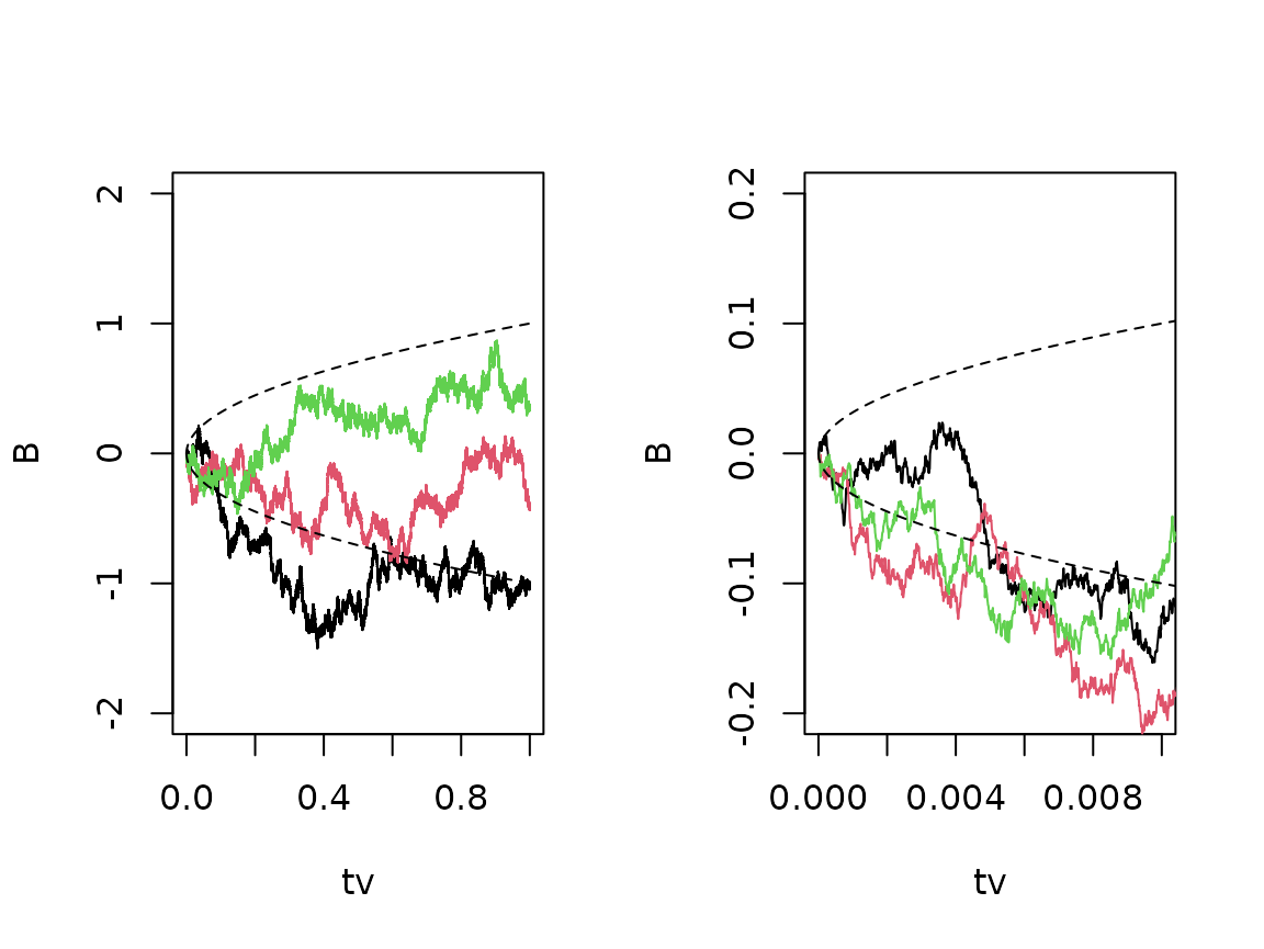

The Brownian bridge

Given two end points, we can simulate a Brownian bridge that connects them. That is, we simulate a Brownain motion conditionally on the end points. The function rBrownianBridge does this efficiently. Here, we sumliate a large number of bridges, and plot only the first few:

  tv <- 10:20
  n <- 1e4
  B0T <- c(15,5)
  sigma <- 2
  BB <- replicate(n,rBrownianBridge(tv,sigma=sigma,B0T=B0T))
  
  matplot(tv,BB[,1:10],type="l",lty=1)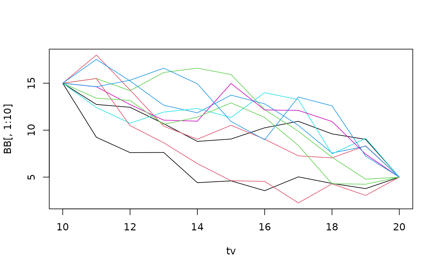

We can verify the statistics by plotting the mean and variance of the bridge. We compare with the analytical results: The expectation follows a straight line connecting the end points, and the variance is a quadratic, which vanishes at the end points and has slope \(\pm 1\) at the end points.

par(mfrow=c(1,2))
plot(tv,apply(BB,1,mean),xlab="t",ylab="mean")
lines(range(tv),B0T)
plot(tv,apply(BB,1,var),xlab="t",ylab="var")
lines(tv,sigma^2*(tv-tv[1])*(1-(tv-tv[1])/diff(range(tv))))

Simulation of the maximum of Brownian motion

We study the maximum of the Brownian motion over a given time interval. We have the analytical result:

\[ \mathbf{P}(S_t \geq x) = 2\mathbf{P}( B_t \geq x) \]

where

\[ S_t= \max\{ B_s : 0\leq s \leq t \} \]

The following code simulates a number of sample paths of Brownian motion \(B_t\) over a time interval \(t=0,\ldots,Nt\). For each sample path we compute the maximum. We plot the the empirical statistics of the maximum against the analytical result. The statistics are the histogram, which should be compared with the probability density function (pdf), and the complementary cumulated distribution function (ccdf), also referred to as the survival function.

require(SDEtools)

hist.maxBM.compare.analytical.Monte.Carlo <- function(Nt,Np)
{ 
  ## Simulate Np trajectories of BM on {0,1,...,Nt}
  B <- rvBM(0:Nt,Np)
  
  ## Compute max(B) 
  maxB <- apply(B,2,max)

  ## Histogram of max(B) vs theoretical p.d.f.  
  hist(maxB,freq=FALSE,xlab="x",ylab="P.d.f.",
       main="Pdf of max(BM)")
  plot(function(x)2*dnorm(x,sd=sqrt(Nt)),from=0,to=max(maxB),add=TRUE)

  ## Empirical vs. theoretical survival function of max(B)
  plot(sort(maxB),seq(1,0,length=Np),type="s",xlab="x",ylab="Ccdf, P(X>x)",
       main="Ccdf of max(BM)")
  plot(function(x)2-2*pnorm(x,sd=sqrt(Nt)),from=0,to=max(maxB),add=TRUE)
}

We first try the comparison using 1000 sample paths (which is sufficient) and over 1000 time steps:

hist.maxBM.compare.analytical.Monte.Carlo(Nt=1000,Np=1000)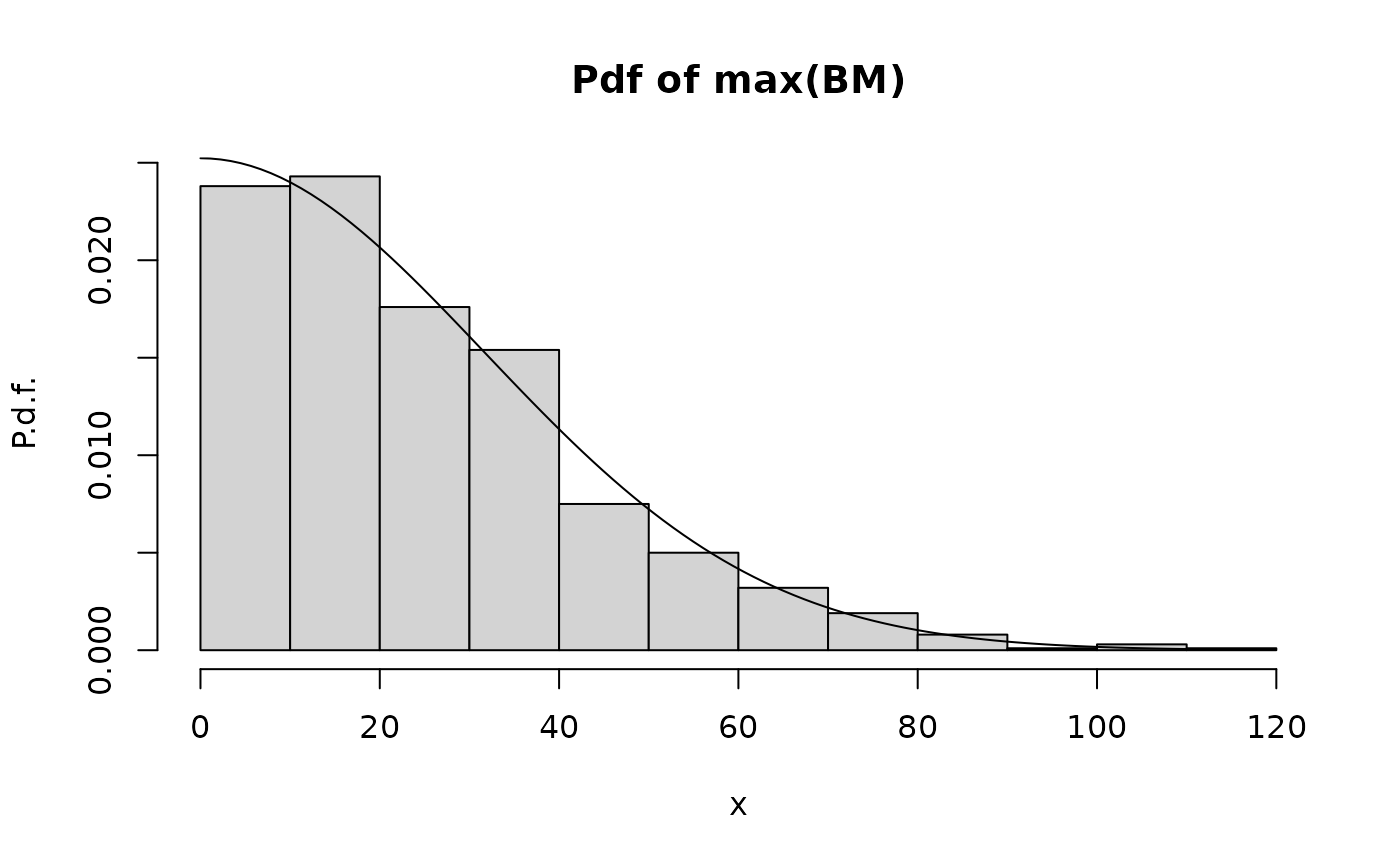

We see that there is excellent agreement between the maximum and the theoretical prediction.

The next graph repeats this for a small number of time steps, \(N_t=10\).

hist.maxBM.compare.analytical.Monte.Carlo(Nt=10,Np=1000)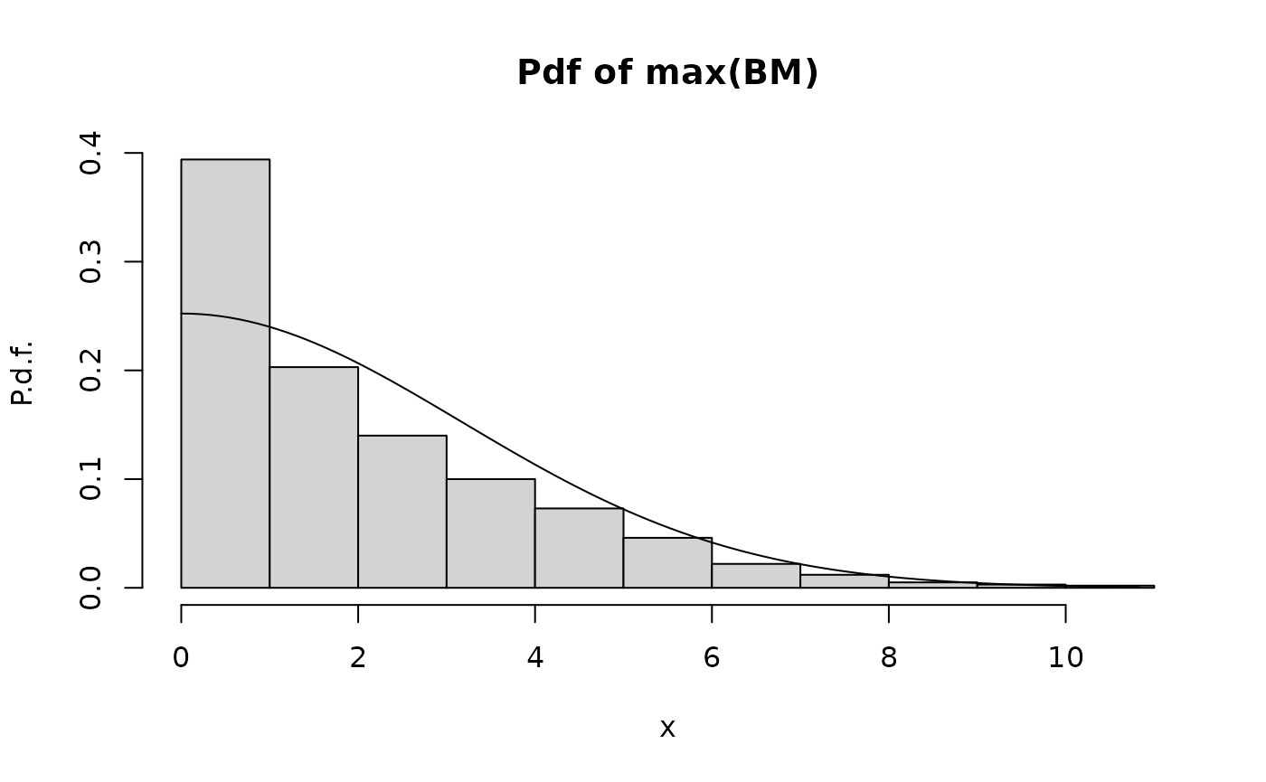

We see that there is poor agreement now. The reason is the difference between the continuous-time maximum

\[ \max\{ B_s : 0 \leq s \leq t\} \]

and the maximum of the sampled process

\[ \max\{ B_s : s=0,1,\ldots,t\} \]

When \(t\) is small, this difference becomes more important.

References

Thygesen, Uffe Høgsbro. 2023. Stochastic Differential Equations for Science and Engineering. Taylor & Francis. http://uffe-h-thygesen.github.io.