The Cox-Ingersoll-Ross process
Uffe Høgsbro Thygesen
2025-12-05
Source:vignettes/CoxIngersollRoss.Rmd
CoxIngersollRoss.RmdThe Cox-Ingersoll-Ross process is given by the Itô stochastic differential equation
We assume that all parameters (, , ) are positive, and that the initial condition is non-negative.
The process is interesting from the point of view of SDE theory, due to the state-dependent noise intensity (). From an applied point of view, the process is popular e.g. to model interest rates. See (Thygesen 2023) for details.
The process remains non-negative. Its expectation satisfies the linear ordinary differential equation which has the solution . Its variance satisifies the equation from which we can derive (Thygesen 2023) e.g. that in stationarity the mean is , the variance is , and the autocovariance function is .
Functionality in SDEtools for the Cox-Ingersoll-Ross process
The SDEtools package has implemented four functions which all relate to the transition probabilities in the Cox-Ingersoll-Ross process. These are dCIR, pCIR, qCIR, rCIR. They follow the convention for other distributions such as the Gaussian (normal) distribution; i.e., dCIR computes transition probability densities, pCIR computes the probability distribution function, qCIR computes quantiles, and rCIR generates random numbers.
They all require as parameters the initial point , the parameters , and , and the terminal time . By default they use the Itô interpretation, but they can optiionally use the Stratonovich interpretation (see details in the following). Finally, they take the usual arguments for similar distributions in R, i.e., probabilities can be natural (default) or logarithmic, and probabilities can concern the lower tail (default) or the upper.
Basic use of the functions
The help file for the functions has the following example: We first sample a number of random numbers, taking all parameters to 1. We plot the p.d.f., and the c.d.f., and verify the consistency between the c.d.f. and the quantile functions.
## Loading required package: SDEtools
example(dCIR)##
## dCIR> x <- sort(rCIR(100,1,1,1,1,1))
##
## dCIR> par(mfrow=c(1,2))
##
## dCIR> plot(x,dCIR(x,1,1,1,1,1),ylab="p.d.f.")##
## dCIR> F <- pCIR(x,1,1,1,1,1)
##
## dCIR> plot(x,F)
##
## dCIR> lines(qCIR(F,1,1,1,1,1),F)
Verifying the stationary distribution
The stationary distribution can be obtained numerically by setting the terminal time to .
We have already mentioned that the stationary mean is and that the stationary variance is . Theoretically, it can be shown that the stationary distribution is a gamma distribution with shape parameter and rate parameter .
The following code verifies this. Note that the argument x0 is still required, but that it can be chosen arbitrarily, as it does not affect the stationary distribution.
  lambda <- 1
  xi <- 1
  gamma <- 1
  x0 <- 1
  t <- Inf

  phi <- function(x) dCIR(x,x0,lambda,xi,gamma,t)
  plot(phi,from=0,to=3)

  Sigma <- gamma^2*xi/(2*lambda)
  k <- xi^2/Sigma
  r <- xi/Sigma
  phi.theo <- function(x) dgamma(x,shape=k,rate=r)
  plot(phi.theo,from=0,to=3,col="red",add=TRUE)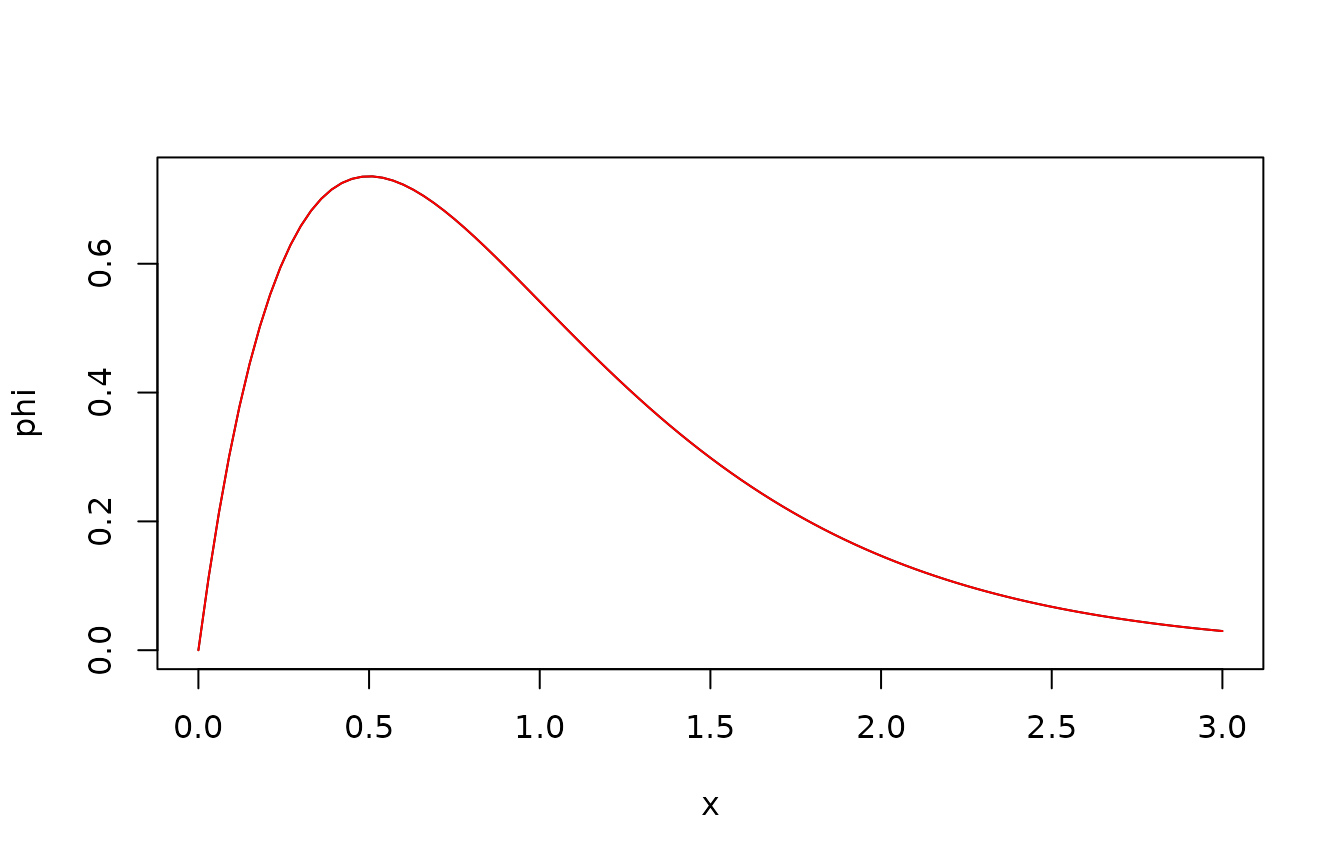
Recursive sampling of a path
We can sample a path of the CIR process recursively, using the Markov property:
  dt <- 0.1
  t <- seq(0,1000,dt)
  X <- numeric(length(t))
  X[1] <- xi

  for(i in 2:length(X)) X[i] <- rCIR(1,X[i-1],lambda,xi,gamma,dt)
  plot(t,X,type="l",xlim=c(0,100))
Verification of the autocovariance function
Here, we compute the empirical autocovariance function based on the simulated sample path. This assumes stationarity, which does not strictly hold, since the initial condition was deterministic () rather than sampled from the stationary distribution. However, the process decorrelates fairly quickly (in fact, over the time scale ), so it is a reasonable approximation.
We compare with the analytical expression for the autocovariance function, . Note that the R function acf by default computes the autocorrelation function (rescaled to have 1 at lag 0), and operates in discrete time (number of samples).
  acf(X,lag.max = 50,type="covariance")
  hv <- 0:50  # Number of samples, not continuous time
  lines(hv,gamma^2/2/lambda*xi*exp(-hv*dt))
Note that there is a clear resemblance between the empirical and the theoretical result, but that the agreement is far from perfect: The variability in the process itself implies that also the estimated autocovariance function is uncertain.
The Stratonovich interpretation
As mentioned, the default interpretation is Itô’s. If one wishes the Stratonovich interpretation, this can be supplied by an optional argument:
dCIR(1,1,1,1,1,1,Stratonovich = TRUE)## [1] 0.6184781Under the hood, the functions immediately transform to the Itô interpretation. The same process can be written either as a solution to an Itô SDE or a Stratonovich SDE using the general rules for converting between the two formalisms (Thygesen 2023):
Note that the both equations have the same structure, the same rate parameter , and the same noise intensity , but that the constant terms are different. So with the Stratonovich interpretation, the stationary expectation is We can verify this by numerical integration, here using the complementary c.d.f.:
  G <- function(x) pCIR(x,x0,lambda,xi,gamma,Inf,Stratonovich = TRUE,lower.tail = FALSE)
  EX <- integrate(G,lower=0,upper=Inf)$value
  plot(G,from=0,to=3,main=paste("Integral=",
                                round(EX,3),"; theoretical=",
                                round(xi+gamma^2/4/lambda,3)))