HMM filtering of scalar SDEs
Uffe Høgsbro Thygesen
2025-12-05
Source:vignettes/HMM-filtering-of-scalar-SDEs.Rmd
HMM-filtering-of-scalar-SDEs.RmdOverview
We simulate a sample path from the Ito stochastic differential equation (Thygesen 2023) governing the abundance of a bacterial population
which is the Cox-Ingersoll-Ross model (Thygesen 2023). Then, we simulate random measurements taken at times so that is Poisson distributed with mean $v `. X_{t_i}$. Then, we pretend that we don’t know the states and re-estimate them from these measurements. We do this with the function , so that this vignette is essentially a demonstration of this function and its use.
Simulation of states
We define the model and simulate the states using the Euler-Maruyama method.
## Loading required package: SDEtools
  set.seed(1234) ## For reproducible results

  # Define model. Note abs to handle negative x.
  gamma <- 1
  f = function(x) (1-x)
  g = function(x) gamma * sqrt(abs(x));

  ## Time vector for simulation
  dt = 0.001;
  Tmax = 20;

  tvec = seq(0,Tmax,dt)
  nt <- length(tvec)

  ## Initial condition, chosen somewhat arbitrarily
  x0 <- 0.1

  ## Enforce that the simulated state should be non-negative
  p <- function(x) abs(x)

  ## Simulate states
  sim <- euler(f,g,tvec,x0,p=p)

  plot(sim$times,sim$X,type="l",xlab="Time",ylab='Abundance')
Simulation of measurements
Next, we generate some random measurements. Measurements are taken at regular points in time; not at every time point where are state values is simulated. We use a Poisson distribution for the measurements. This correspond to a situation where we count the number of individuals in a small sample from the environment.
## Generate random measurements
  tsample <- 0.1
  vsample <- 1

  sampleIndeces <- round(seq(1,length(tvec),(tsample/dt)))
  tm = tvec[sampleIndeces];
  xtrue <- sim$X[sampleIndeces]
  ymean = vsample * xtrue

  # Generate random measurements
  ymeas <- rpois(length(tm),lambda=ymean)

  plot(sim$times,sim$X,type="l",xlab="Time",ylab='Abundance')
  points(tm,ymeas/vsample,pch='o')
Notice that the data is very noisy and, when plotted in this fashion, does not seem to hold very accurate information about the state.
Specification of the state likelihood function
To run the filter, we must first specify the state likelihood function. We first define this for a general measurement and general state:
  ## State likelihood
  dl <- function(x,y) dpois(y,lambda=vsample*x)
We can now inspect the state likelihood on its own, i.e., without using the process equation. We choose a discretization of state space which has higher resolution near 0, and tabulate the likelihood function.
  ## Choose discretization of state space
  xi <- seq(0,3,0.025)^2                                # Cell Interfaces
  xc <- cell.centers(xi)

  ltab <- outer(xc,ymeas,dl)
  image(tm,xc,t(ltab),xlab="Time",ylab="State")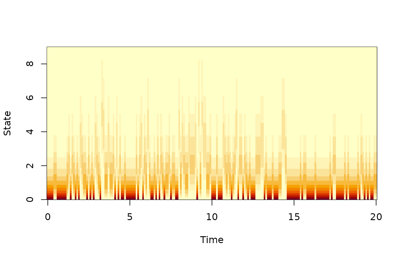
We plot the most likely state, given just the measurements, on top of the true states:

Again, there is very little information in the individual observation, because the counts are so low. Therefore, there is a potential gain from estimating the state not just using the measurement taken at the same time, but also the neighbouring measurements. This is particularly so because the measurements are taken quite frequently: The sample interval is 0.1 time unit, while the mean relaxes over a time scale of 1.
Running the filter
We now use the filter to add the information from the process equation. We use the function , which requires a process model as well as a state likelihood function. In addition, it needs a distribution of the initial state. We focus first on real-time state estimation; i.e., we use only the current and past measurements in the estimation, not future measurements.
  # Advection-diffusion form of the Kolmogorov equations
  D = function(x) 0.5*gamma^2*x;
  u = function(x) f(x) - 0.5*gamma^2;

  ## Specify prior c.d.f. of the initial state, here uniform. Note that it does not have to be normalized.
  phi0 <- function(x)x
  ## Run the filter
  filter <- HMMfilterSDE(u,D,xi,bc='r',phi0,tm,ymeas,dl,
                         do.Viterbi=TRUE,do.smooth=TRUE,N.sample = 3)
## Loading required package: Matrix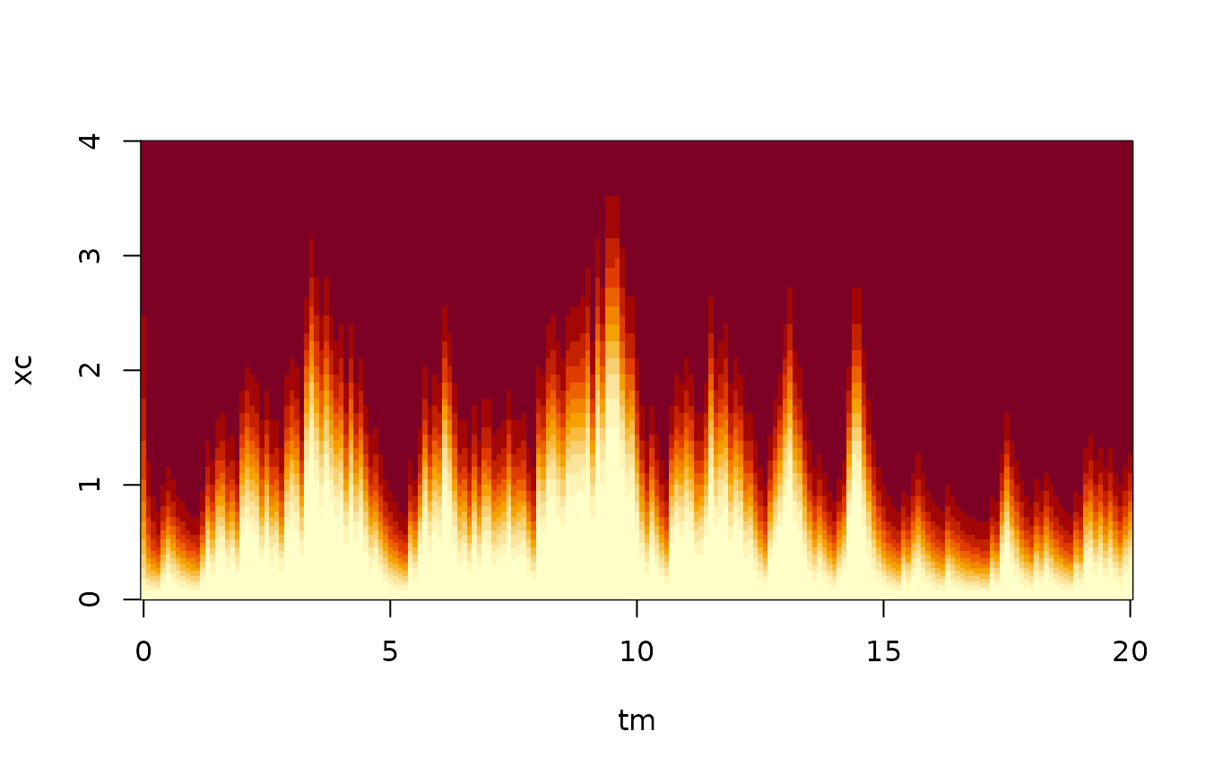
Filtering results
We compare the true states with the estimated ones:
  ## Plot true state at times of measurements
  plot(tm,ymean/vsample,type="l",xlab="t",ylab="x")

  ## Compute and plot posterior mean
  XestMean <- filter$psi %*% xc
  points(tm,XestMean)
Notice how, as anticipated, the estimated states lag a bit behind the true ones, and that some of the fast fluctuations in the true states do not reflect in the estimated ones.
We compute the variance in the posterior distribution, at each point in time:

Notice how the variance fluctuates significantly in time. This reflects that both the process equation and the measurement equation has a variance, which depends on the state. To pursue this further, we can compare the mean and the variance in the posterior distribution:
plot(XestMean,XestVar)
Note that there seems to be a roughly linear relationship (save the first couple of data points, which reflect transients from the initial condition). This linear relationship reflects both process noise and measurement noise: When the state is large, the process noise is increased, and the variance on the measurements is larger.
The smoothing filter
The filter algorithm outputs both the predicted, estimated, and smoothed distributions of the state. We now compare how different information yield different estimates.
  XpredMean <- filter$phi %*% xc
  XpredVar <- filter$phi %*% xc^2 - XpredMean^2

  XsmoothMean <- filter$pi %*% xc
  XsmoothVar <- filter$pi %*% xc^2 - XsmoothMean^2

  plot(sim$t,sim$X,type="l",xlab="t",ylab="x")
  lines(tm,XsmoothMean,col="red")
  lines(tm,XestMean,col="blue")
  legend("topright",lty=1,col=c("black","red","blue"),legend=c("True","Smooth","Est"))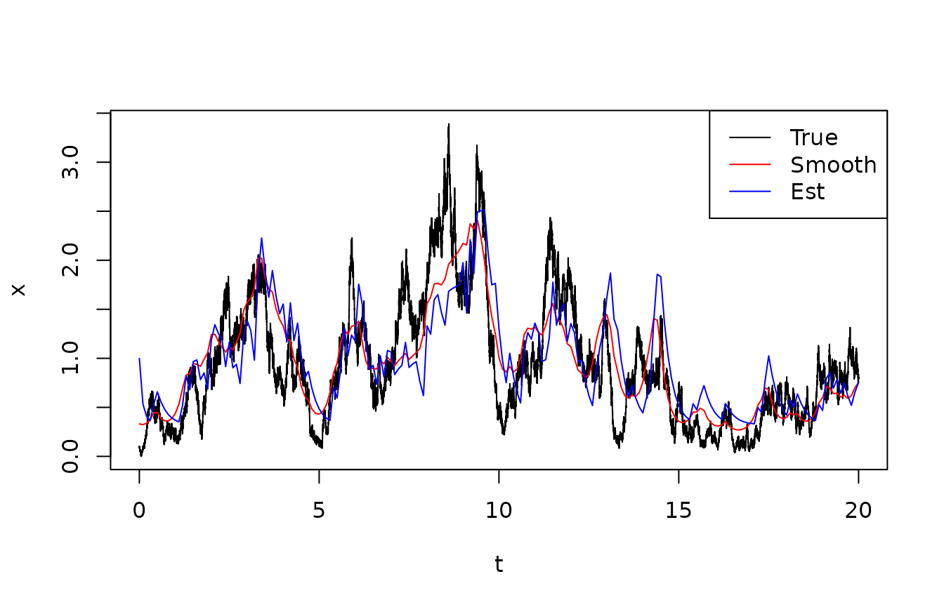
Notice that the difference between the estimated state and the smoothed state is not very large. In the time interval , the smoother is a bit ahead of the estimator. This is because the true state largely keeps increasing over this time interval, which keeps surprising the estimator, but which the smoother takes into account.
We can compare the time-averaged variances between the three state estimates (predicted, estimated, smoothed). We do this in two ways: First, we compute the variance in the posterior distributions - this is the way one would assess variance in e real situation, where the true states are not available. Second, we compute the time averaged square deviation between the estimated states and the true ones. This is clearly only possible since this is a simulation exercise where we know the truth.
Theo <- c(Pred = mean(XpredVar),Est = mean(XestVar),Smooth = mean(XsmoothVar))
Emp <- c(mean((XpredMean-xtrue)^2),
             mean((XestMean-xtrue)^2),
             mean((XsmoothMean-xtrue)^2))

Vars <- rbind(Theo,Emp)
print(Vars)
## Pred Est Smooth
## Theo 0.2954795 0.2082373 0.1449298
## Emp 0.3369900 0.1850625 0.1118570The different between the theoretical variances and the empirical ones are reasonable and do not show a clear pattern. The difference between predictions, estimates, and smoothed estimates reflect that more data points are being used to form the estimates, resulting in a lower variance.
The most probable path
The output from the filter included the most probable path, that is, the sequence of states which maximize the joint posterior probability. This is found with the Viterbi algorithm. The following figure shows the true state, the posterior expectation (based on the smoothing filter, and the most probable path).
plot(sim$t,sim$X,type="l",xlab="t",ylab="x")
lines(tm,XsmoothMean,col="red")
lines(tm,filter$Xmpt,col="blue")
legend("topright",lty=1,col=c("black","red","blue"),legend=c("True","Smooth","MPT"))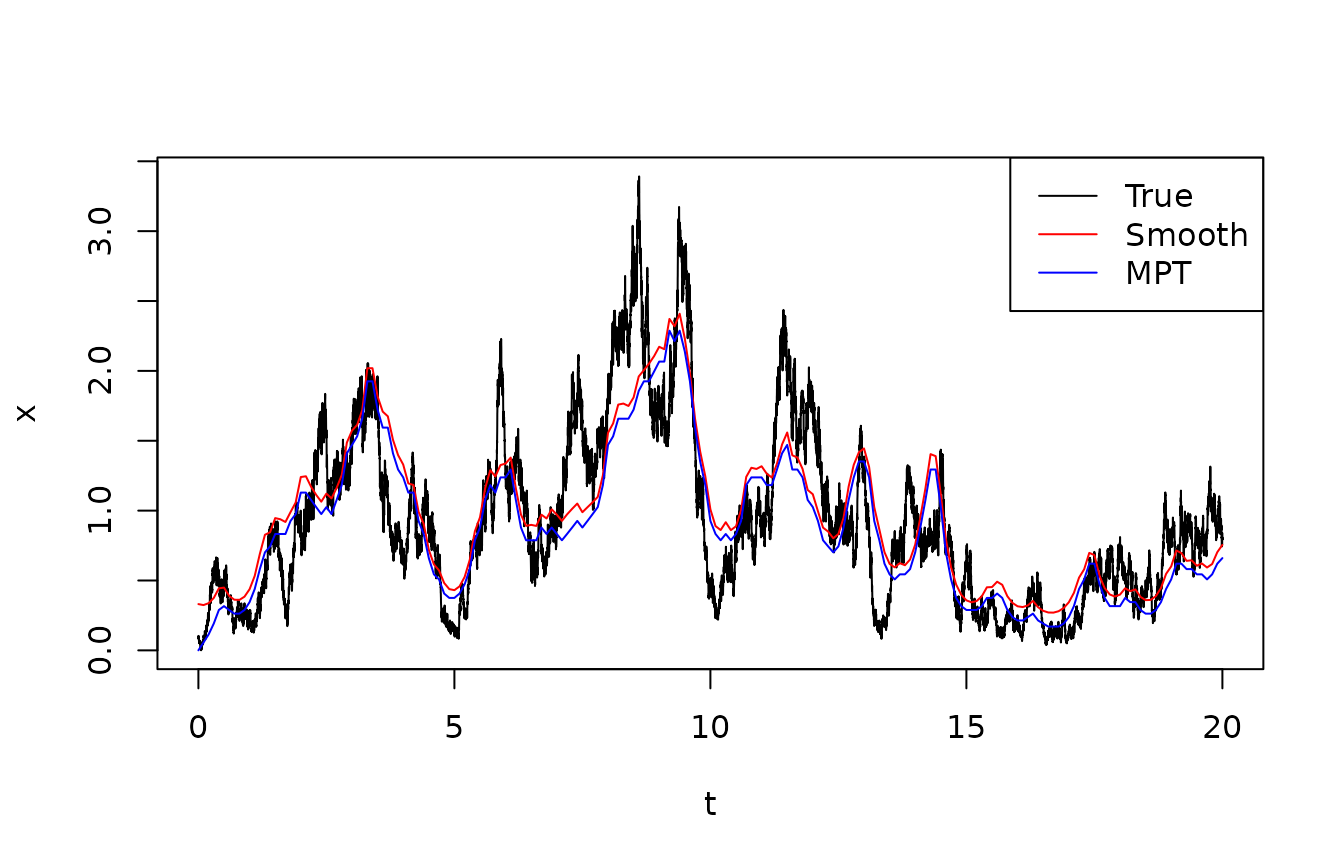
In this example, there is not a very pronounced difference between the smoothed mean and the most probable track. The most probable track is systematically slightly below the mean, which is unsurprising given the skewness in the posterior distributions. However, conceptually there is quite a big difference in the way they are formed, and if they differ significantly, this should lead to a closer inspection.
Sampling typical tracks
It is often useful to sample “typical tracks” from the posterior, i.e., entire state sequences from their joint distribution. These can be used both to communicate the filter results, and in particular, the uncertainty on the estimated tracks. Non-specialists often find such simulated tracks more informative than confidence intervals. Also, the simulated tracks hold information about conditional autocovariance which is not captured by the marginal posterior distributions provided by the smoothing filter, so they can be used for Monte Carlo estimation of statistics such as the posterior probability that the state enters a given region.
The following code compares the true track with the Most Probable Track and a few (3) simulated typical tracks from the posterior.
plot(sim$t,sim$X,type="l",xlab="t",ylab="x")
matplot(tm,filter$Xtyp,col="red",type="l",add=TRUE)
lines(tm,filter$Xmpt,col="blue")
legend("topright",lty=1,col=c("black","red","blue"),legend=c("True","Typical","MPT"))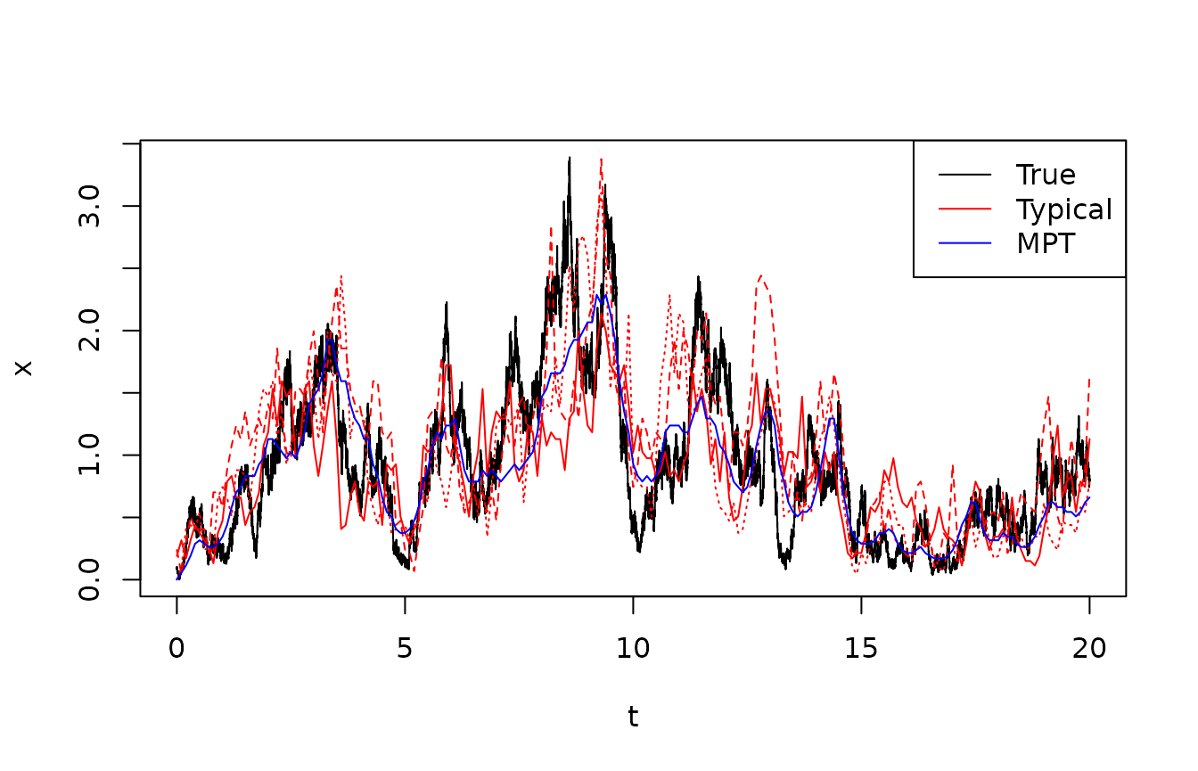
Perspectives
It is possible to estimate the states between the measurements, for example by having a state likelihood function which is constant to 1 whenever no measurement is taken. Then, you could investigate how the posterior variance evolves between times of measurements.
The function gives various output that can be used to assess model fit: The total log-likelihood can be used in an “outer loop” to estimate model parameters using the Maximum Likelihood principle, and describes how well, on average, the model does one-step predictions. The normalization constants apply to each time step, and can be used to identify observations that were very unexpected, and therefore potential outliers. This can be refined using the prediction pseudo-residuals , which theoretically should be independent and uniformly distributed on [0,1]; this can be used for model validation.