Verifying Itô’s formula through simulation
Itô’s formula, in its simplest version, states that when and is an Itô process Moreover, the quadratic variation is given by , so See (Thygesen 2023) for a description of this theoretical result.The aim of this vignette is to verify this numerically for a specific example, and to discuss discretization errors when we verify the formula in discrete time.
In our example, is stochastic logistic growth given by the Itô stochastic differential equation with and the initial condition . This is known as stochastic logistic growth (Thygesen 2023). We simulate a sample path of using the Euler-Maruyama algorithm:
## Loading required package: SDEtools
  set.seed(123456)

  f <- function(x) x*(1-x)
  g <- function(x) sigma*x

  t <- seq(0,10,0.01)
  B <- rBM(t)
  x0 <- 0.01
  sigma <- 0.25
  X <- euler(f,g,t,x0,B)$X

  plot(t,X,type="l")
We now map this process through the function to generate :

We now verify the first variant of Itô’s formula, viz. We first generate the quadratic variation , and then perform numerical Itô integration:
qvX = QuadraticVariation(X)
Y1 <- h(x0) + itointegral(hp(X),X) + 0.5*itointegral(hpp(X),qvX)

plot(t,Y,type="l")
lines(t,Y1,col="red")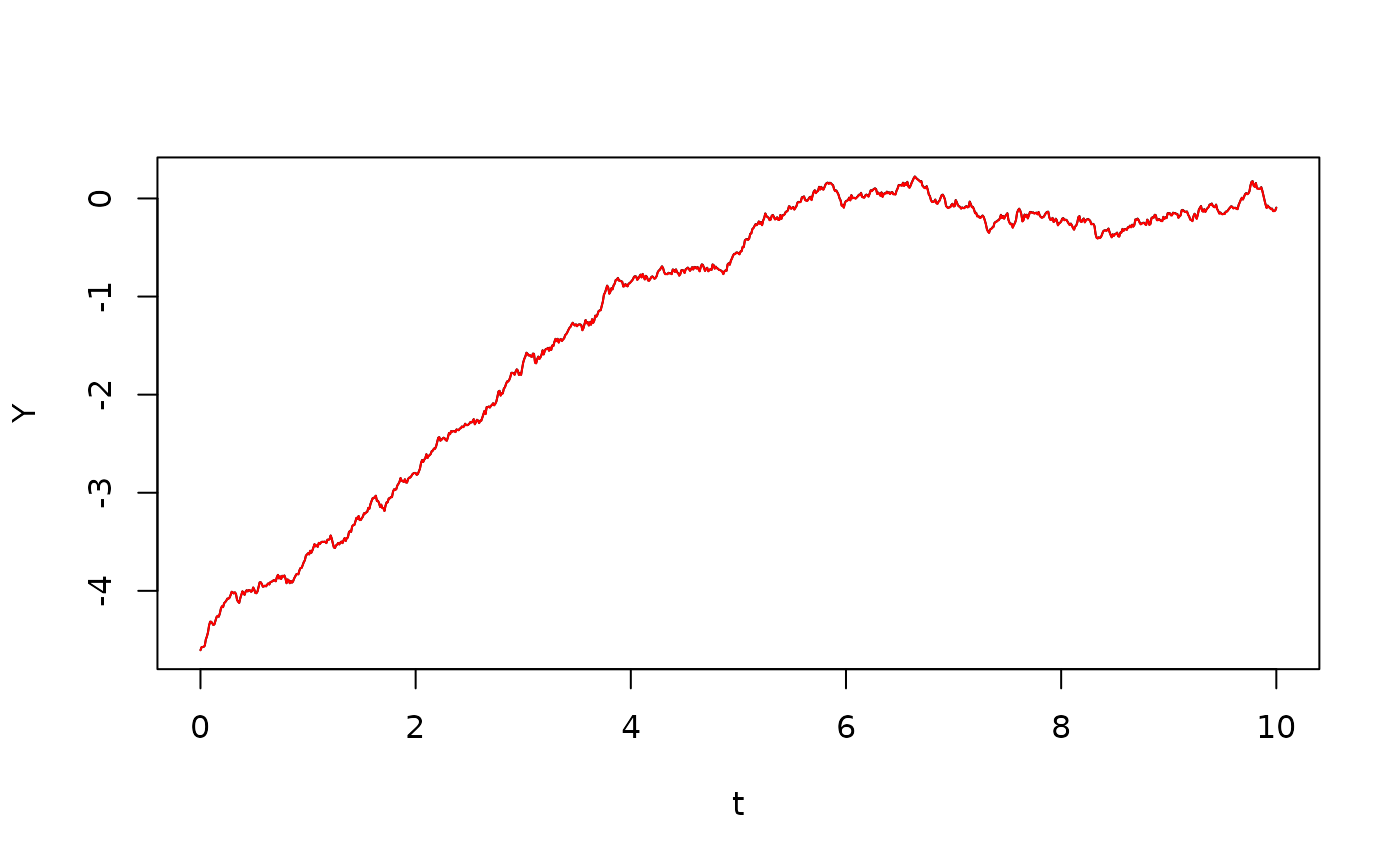
The two lines lie nicely on top of each other, but there is some discretization error. We will look at this error later.
We now do the same for the second formulation, where we use the result .
Y2 <- h(x0) + itointegral(hp(X),X) + 0.5*itointegral(hpp(X)*g(X)^2,t)

plot(t,Y,type="l")
lines(t,Y2,col="green")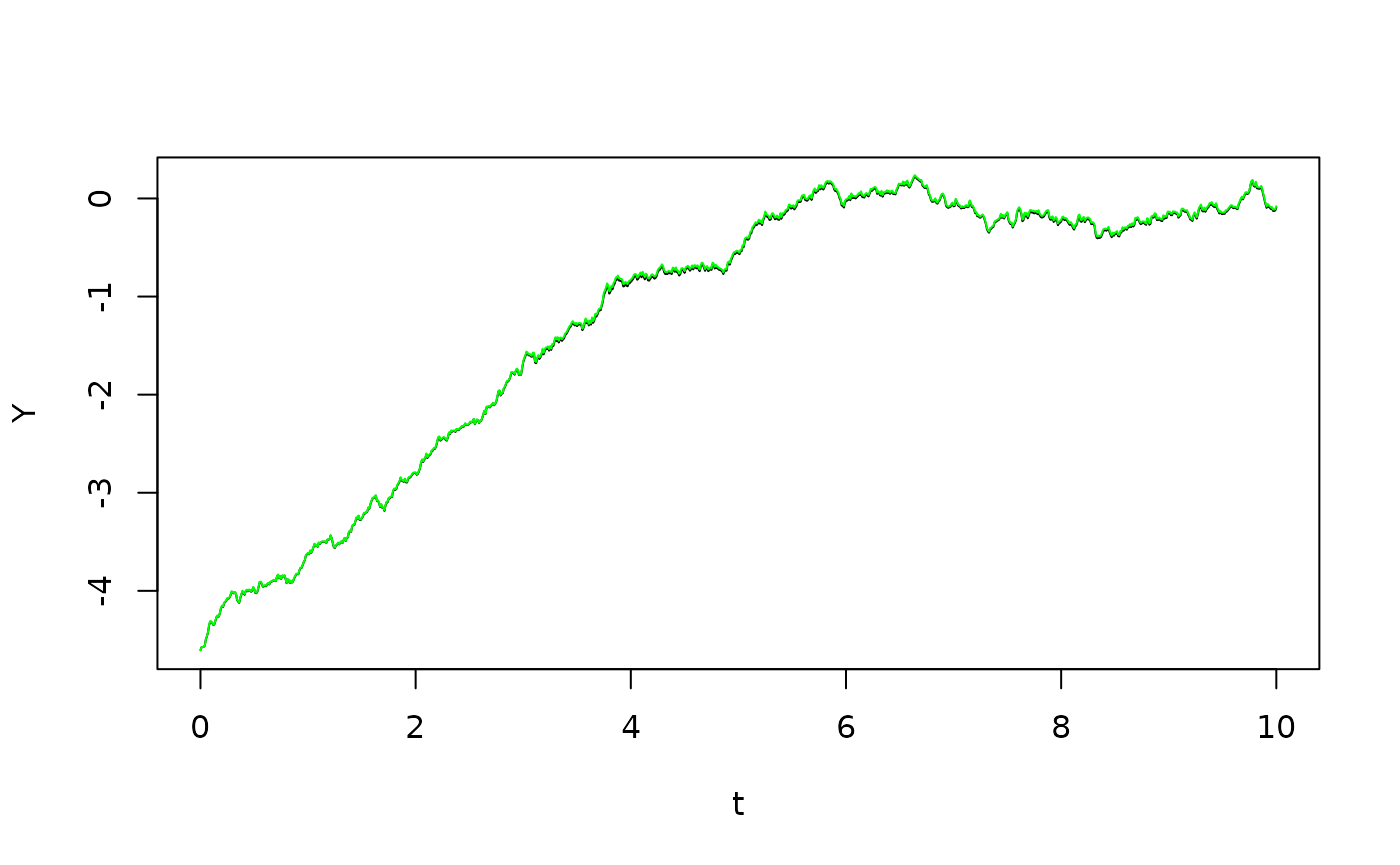
Again we see that the two lines lie on top of each other, although the discretization error in this case appears to be a little more visible.
Next, we could manipulate the integral equation for further. Inserting the forms for , , and , we get
which leads to the following representation of :
Y3 <- h(x0) + itointegral(1-X-0.5*sigma^2,t) + sigma*B

plot(t,Y,type="l")
lines(t,Y3,col="blue")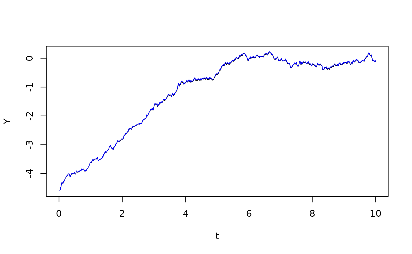
Finally, we can substitute in this expression, thus obtaining an Itô stochastic differential equation for , viz.:
The following code solves this equation and compares with the previous solution:
  fY <- function(y) 1-exp(y)-0.5*sigma^2
  gY <- function(y) sigma
  Y4 <- euler(fY,gY,t,log(x0),B)$X

  plot(t,Y,type="l")
  lines(t,Y4,col="purple")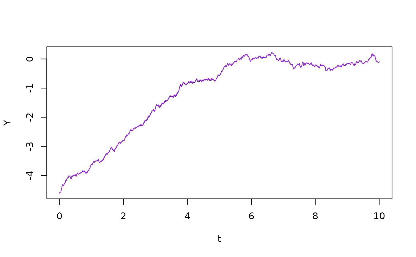
The discretization error
We now examine the discretization error associated with the numerical Itô integration. The first formulation,
leads to a discretization error, because we are effectively truncating at second order in Taylor’s formula when computing increments over each time step:
so that this version of Itô’s formula ignores the higher order terms . We can compute the error:
plot(t,Y-Y1,type="l")
To estimate the error, note from Taylor’s formula that the leading error term is . Here, . During the growth phase, the increment has conditional expectation and variance , so the mean cubed is . As a result, the error should grow with rate per time step, i.e. with a rate . So after 5 time units, the error should be . We see that there is good agreement with the simulation result.
We now consider the discretization error in the second formulation, Here, there is also the effect that the increment in discretized quadratic variation , i.e. , does not exactly equal . In fact, the conditional variance of the increment equals , but in discrete time, there is both a random component and a mean. This error can be traced back the underlying Brownian motion: In discrete time, its quadratic variation does not exactly equal time. In this case, this error turns out to be larger than the one we examined previously:
plot(t,Y-Y2,type="l")
To assess this error coarsely, note that it comes from the term and the conditional expectation of this term is per time step during the growth phase, i.e. it grows with rate . So after 5 time units, we expect that this error has grown to 0.025. We see a good agreement with the simulation, even if the variation between realizations are greater.
This vignette has hopefully illuminated both where Itô’s formula comes from, and the errors that may arise when we investigate stochastic differential equation in discrete time.