The example: An animal moving in one dimension and subject to killing
In this vignette, we consider a process given by the Itô stochastic differential equation
We interpret this as the position of an animal moving in one dimension. The position is an Ornstein-Uhlenbeck process (Thygesen 2023) with stationary mean 0, variance , and decorrelation time 1. We can verify the stationary distribution numerically as follows, introducing reflective boundaries at the boundaries of a computational domain. Here is the diffusivity, and is the advective velocity which equals the drift, since the diffusivity is constant.
## Loading required package: SDEtools
xgrid <- seq(-3,3,length=102)
xc <- cell.centers(xgrid)

v <- function(x) -x
D <- function(x) 0.5

G0 <- fvade(v,D,xgrid=xgrid,bc='r')
## Loading required package: Matrix
pi <- StationaryDistribution(G0)
plot(xc,pi/diff(xgrid),xlab="x",ylab="P.d.f.",type="l")
Constructing the sub-generator of a diffusion with killing
We assume that the animal dies with a killing rate . That is, we have a stopping (killing) time such that the conditional probability of killing in the interval is
Thus, the mortality (killing rate) is higher for greater values of .
The sub-generator associated with this process is given by and includes advection , diffusion , and killing .
We discretize this sub-generator as follows (using reflection at the boundaries):
To verify this sub-generator, we plot the row sums and compare with the killing rate:
xc <- cell.centers(xgrid)
plot(xc,-rowSums(G))
lines(xc,r(xc),col="red")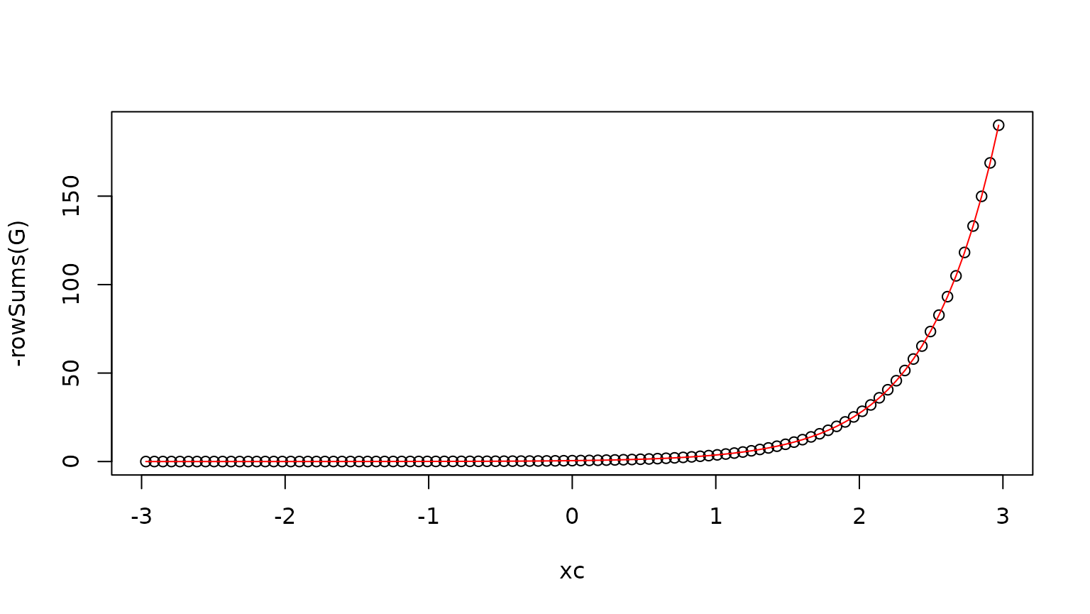
Recall that for the discretized system, a continuous-time Markov chain jumping between computational grid cells, the row sum is minus the rate of leaving the domain, i.e. jumping to the “coffin” state of death.
Finding the distribution at a later time
Assume that the state starts at a given point . At a later time , the probability is distributed partly on the real axis, and partly in the “coffin” state. Here, we compute the probability density over the real axis.
x0 <- 0
phi0 <- diff(xgrid>x0)
phit <- phi0 %*% expm(G)
psurv <- sum(phit)

rhot <- phi0 %*% expm(G0)

plot(xc,rhot,type="l",lty="dashed",main=paste("Probability of survival",psurv))
lines(xc,phit)
legend("topright",legend=c("With killing","Without killing"),lty=c(1,2))
Notice that the killing removes a significant fraction of the probability, in particular from the right part of the distribution, where the mortality is higher.
Finding the expected time spent in each cell
Let denote the probability density that and . We can then find the expected time spent in each state as
This must solve the equation
where is the adjoint of sub-generator, i.e. the forward Kolmogorov equation with killing. In discrete formulation:

The expected time to killing
We can find the expected lifetime by integrating the density w.r.t. :
Etau <- sum(rho)We can compare this with the survival function :
  tv <- seq(0,3*sqrt(Etau),length=25)^2
  Gt <- sapply(tv,function(t) sum(phi0 %*% expm(G*t)))
  plot(tv,Gt,type="l")
  abline(v=Etau,lty="dashed")
Finally we compare the total expected life time as found from , with that found by integrating the survival function:
print(Etau)## [1] 1.689603## [1] 1.697609The error is the due to the discretization of time.
The quasi-stationary distribution
In stationarity, the animal is dead, so the more interesting question is the quasi-stationary distribution:
  pi <- QuasiStationaryDistribution(G)
  plot(xc,pi$vector/diff(xgrid),type="l",
       main=paste("Expected life time",1/pi$value),xlab="x",ylab="P.d.f.")
Notice that the quasi-stationary density is shifted to the left, relative to the stationary distribution without killing, since the surviving animals are found predominantly where the killing rate is low.
Simulation of a trajectory
We can simulate an individual trajectory starting at a given point in space, up to the point of killing, as follows.
f <- function(x) v(x)
g <- function(x) 1

times <- seq(0,6,0.01)
x0 <- 0
Stau <- runif(1)

sim <- SDEtools::euler(f,g,times,x0,r=r,Stau=Stau)

plot(X~times,data=sim,type="l")
Let us use this to verify that the distribution of the life time matches
the exponential distribution, when the initial condition is chosen from
the quasi-stationary distribution.
Let us use this to verify that the distribution of the life time matches
the exponential distribution, when the initial condition is chosen from
the quasi-stationary distribution.
The following code chooses a random initial state, from the quasi-stationary distribution.
  simulate.x0 <- approxfun(c(0,cumsum(pi$vector)),xgrid)

  x0s <- sapply(runif(1000),simulate.x0)
  hist(x0s,freq=FALSE,breaks=50)
  lines(xc,pi$vector/diff(xgrid))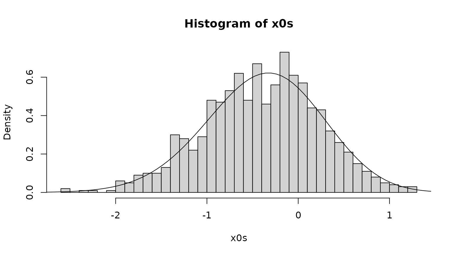
We next simulate a trajectory from each initial position, until death - or , whichever comes first.
simulate.lifespan <- function(x0)
{
sim <- SDEtools::euler(f,g,times,x0,r=r)
return(c(tau=sim$tau,Xtau = tail(sim$X,1)))
}
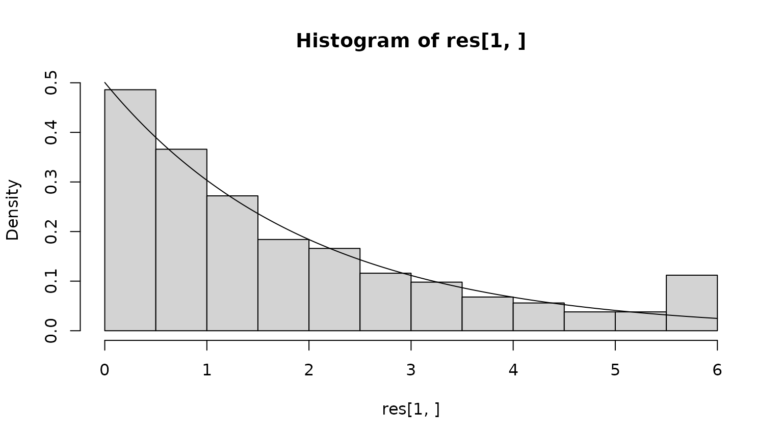
res <- sapply(x0s,simulate.lifespan)We can now compare the observed lifetime distribution with the theoretical prediction, which is an exponential with a rate given by the quasi-stationary distribution.
 Finally, what is the position at depth? We first assess this from the
simulation, excluding those realizations which do not result in death
before the simulation time is over.
Finally, what is the position at depth? We first assess this from the
simulation, excluding those realizations which do not result in death
before the simulation time is over.
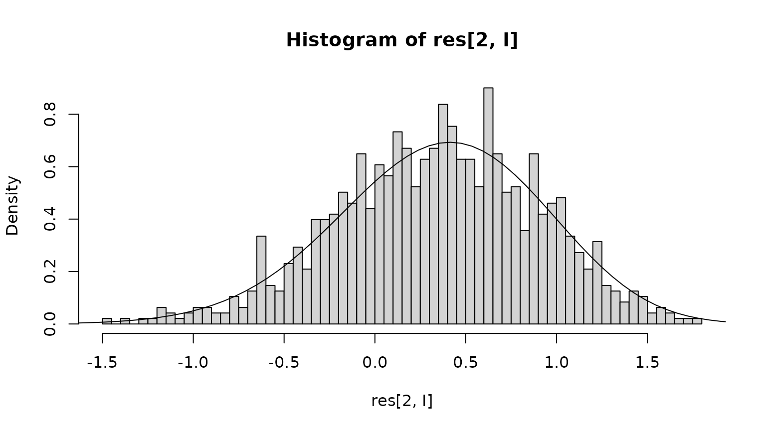
We next compare with the theoretical prediction: At any point in time, conditional on the animal being alive, the state is distributed according to the quasi-stationary distribution . The probability that the animal dies in the next time step is , to first order in the time step , where we condition on the state being . Therefore, using Bayes’ formula, the probability of the state being at , conditional on dying, is proportional to . We compute this and renormalize and compare with the empirical distribution:
  I <- res[1,] < max(times)
  hist(res[2,I],freq=FALSE,breaks=50)
  fXtau <- pi$vector * r(xc)
  fXtau <- fXtau / sum(fXtau)
  lines(xc,fXtau / diff(xgrid))