fvade2d discretizes the advection-diffusion equation
dC/dt = -div ( u C - D grad C)
on a rectangular domain using the finite-volume method. Here, u=(ux,uy) and D=diag(Dx,Dy)
fvade2d(
  ux,
  uy,
  Dx,
  Dy,
  xgrid,
  ygrid,
  bc = list(N = "r", E = "r", S = "r", W = "r"),
  Dxy = function(x, y) 0
)
Arguments
- ux
function mapping state (x,y) to advective term (numeric scalar)
- uy
function mapping state (x,y) to advective term (numeric scalar)
- Dx
function mapping state (x,y) to diffusivity (numeric scalar)
- Dy
function mapping state (x,y) to diffusivity (numeric scalar)
- xgrid
The numerical grid. Numeric vector of increasing values, giving cell boundaries
- ygrid
The numerical grid. Numeric vector of increasing values, giving cell boundaries
- bc
Specification of boundary conditions. See details.
Value
a quadratic matrix, the generator of the approximating continuous-time Markov chain, with (length(xgrid)-1)*(length(ygrid)-1) columns
Details
Boundary conditions: bc is a list with elements N,E,S,W. Each element is either "r": Reflective boundary "a": Absorbing boundary: Assume an absorbing boundary cell, which is not included "e": Extend to include an absorbing boundary cell "p": Periodic. When hitting this boundary, the state is immediately transferred to the opposite boundary, e.g. N->S.
Return value: The function fvade returns a generator (or sub-generator) G of a continuous-time Markov Chain. This chain jumps between cells defined by xgrid and ygrid. When using the generator to solve the Kolmogorov equations, note that G operates on probabilities of each cell, not on the probability density in each cell. The distinction is particularly important when the grid is non-uniform.
Examples
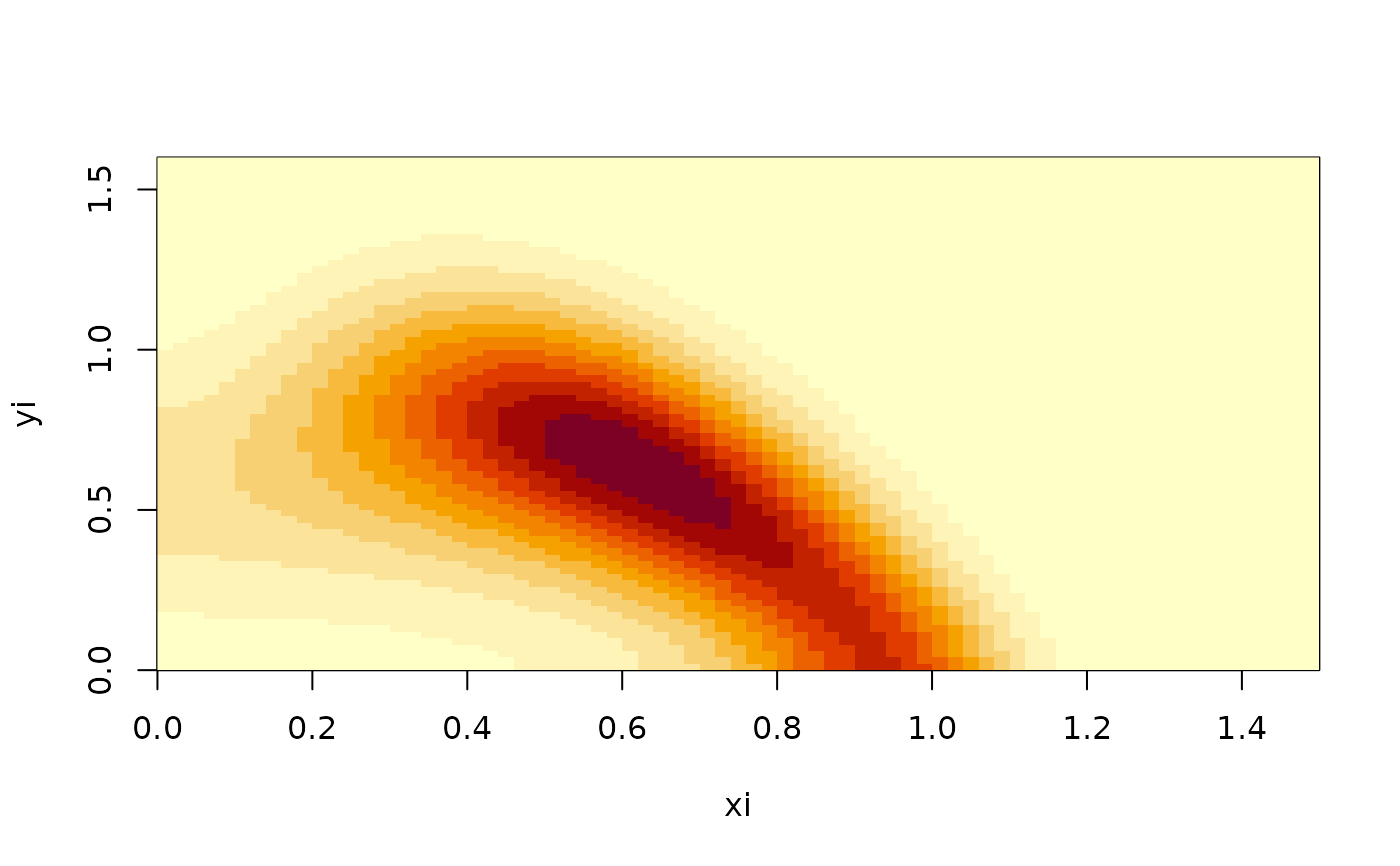
# Generator of a predator-prey model
xi <- seq(0,1.5,0.02)
yi <- seq(0,1.6,0.02)
xc <- 0.5*(utils::head(xi,-1)+utils::tail(xi,-1))
yc <- 0.5*(utils::head(yi,-1)+utils::tail(yi,-1))

ux <- function(x,y) x*(1-x)-y*x/(1+x)
uy <- function(x,y) y*x/(1+x)-y/3
D <- function(x,y) 0.01

G <- fvade2d(ux,uy,Dx=D,Dy=D,xi,yi)

phiv <- StationaryDistribution(G)
phim <- unpack.field(phiv,length(xc),length(yc))
image(xi,yi,t(phim))