Heun's method for simulation of a Stratonovich stochastic differential equation dX = f dt + g dB

Heun's method for simulation of a Stratonovich stochastic differential equation dX = f dt + g dB

heun(
  f,
  g,
  times,
  x0,
  B = NULL,
  p = function(x) x,
  h = NULL,
  r = NULL,
  S0 = 1,
  Stau = runif(1)
)

Arguments

f

function f(x) or f(t,x) giving the drift term in the SDE

g

function g(x) or g(t,x) giving the noise term in the SDE

times

numeric vector of time points, increasing

x0

numeric vector giving the initial condition

B

sample path of (multivariate) Browniań motion. If omitted, a sample is drawn using rvBM

p

Optional projection function that at each time poins projects the state, e.g. to enforce non-negativeness

h

Optional stopping function; the simulation terminates if h(t,x)<=0

Examples

times <- seq(0,10,0.1)

# Plot a sample path of the solution of the SDE dX=-X dt + dB
plot(times,heun(function(x)-x,function(x)1,times,0)$X,type="l")


# Plot a sample path of the solution of the 2D time-varying SDE dX=(AX + FU) dt + G dB

A <- array(c(0,-1,1,-0.1),c(2,2))
F <- G <- array(c(0,1),c(2,1))

f <- function(t,x) A %*% x + F * sin(2*t)
g <- function(x) G

BM <- rBM(times)

plot(times,heun(f,g,times,c(0,0),BM)$X[,1],type="l")

# Add solution corresponding to different initial condition, same noise

lines(times,euler(f,g,times,c(1,0),BM)$X[,1],type="l",lty="dashed")


# Solve geometric Brownian motion as a Stratonovich equation
times <- seq(0,10,0.01)
BM <- rBM(times)
plot(times,heun(function(x)-0.1*x,function(x)x,times,1,BM)$X,type="l",xlab="Time",ylab="X")

# Add solution of corresponding Ito equation
lines(times,euler(function(x)0.4*x,function(x)x,times,1,BM)$X,lty="dashed")


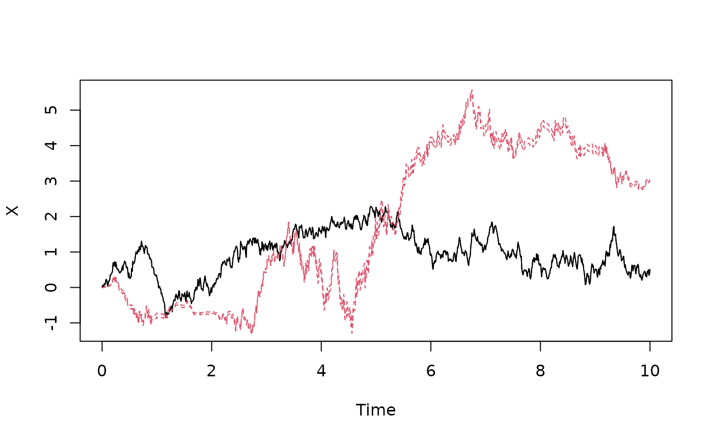
# Testing a case with non-commutative noise
BM2 <- rvBM(times,2)
matplot(times,heun(function(x)0*x,
  function(x)diag(c(1,x[1])),times,c(0,0),BM2)$X,xlab="Time",ylab="X",type="l")

# Add solution to the corresponding Ito equation
matplot(times,euler(function(x)0*x,
  function(x)diag(c(1,x[1])),times,c(0,0),BM2)$X,xlab="Time",ylab="X",type="l",add=TRUE)